Continuum data reduction using CASA

The tutorial is intended to provide you an introduction to the basic steps involved in the analysis of continuum data from the GMRT. We will be using a band-4 (550 - 750 MHz) dataset.

CASA version used for the tutorial: 6.5.2

Introduction

You need to have CASA installed on your machine. You also need the data to be available on your disk.

From the GMRT online archive you can download data in “lta” or “FITS” format. If you downloaded the data in lta format then you will need to do the following steps to convert it to FITS format. You can download the pre-compiled binary files “listscan” and “gvfits” from the observatory.

LTA to FITS conversion

listscan fileinltaformat.lta

At the end of this a file with extension .log is created. The next step is to run gvfits on this file.

gvfits fileinltaformat.log

The file TEST.FITS contains your visibilities in FITS format. Before running gvfits, you can edit the fileinltaformat.log and provide a name of your choice in place of TEST.FITS.

FITS to MS conversion

At this stage start CASA using the command casa on your terminal. You will be on the Ipython prompt and a logger window will appear. The remaining analysis will be done at the CASA Ipython prompt. We use the CASA task importgmrt to convert data from FITS to MS format. In our case the FITS file is already provided so we proceed with that FITS file.

casa
inp importgmrt
fitsfile='SGRB-DATA.FITS'
vis='multi.ms'
go importgmrt

The output file multi.ms file will contain your visibilities in MS format.

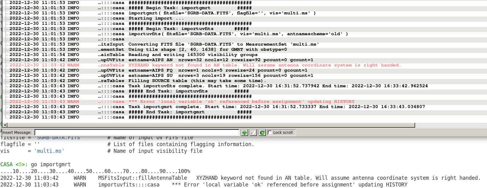
Output of the task importgmrt in the logger and view of the terminal. We will ignore the warnings in the logger for this tutorial.

An alternative way to run the task is as follows:

importgmrt(fitsfile=''SGRB-DATA.FITS',vis='multi.ms')

For the tutorial, we will follow the first method.

The MS format stores the visibility data in the form of a table. The data column contains the data. Operations like calibration and deconvolution will produce additional columns such as the corrected and model data columns.

Data inspection

You will first want to know about the contents of the MS file. The task listobs will provide a summary of the contents of your dataset in the logger window.

inp listobs
vis='multi.ms'
go listobs

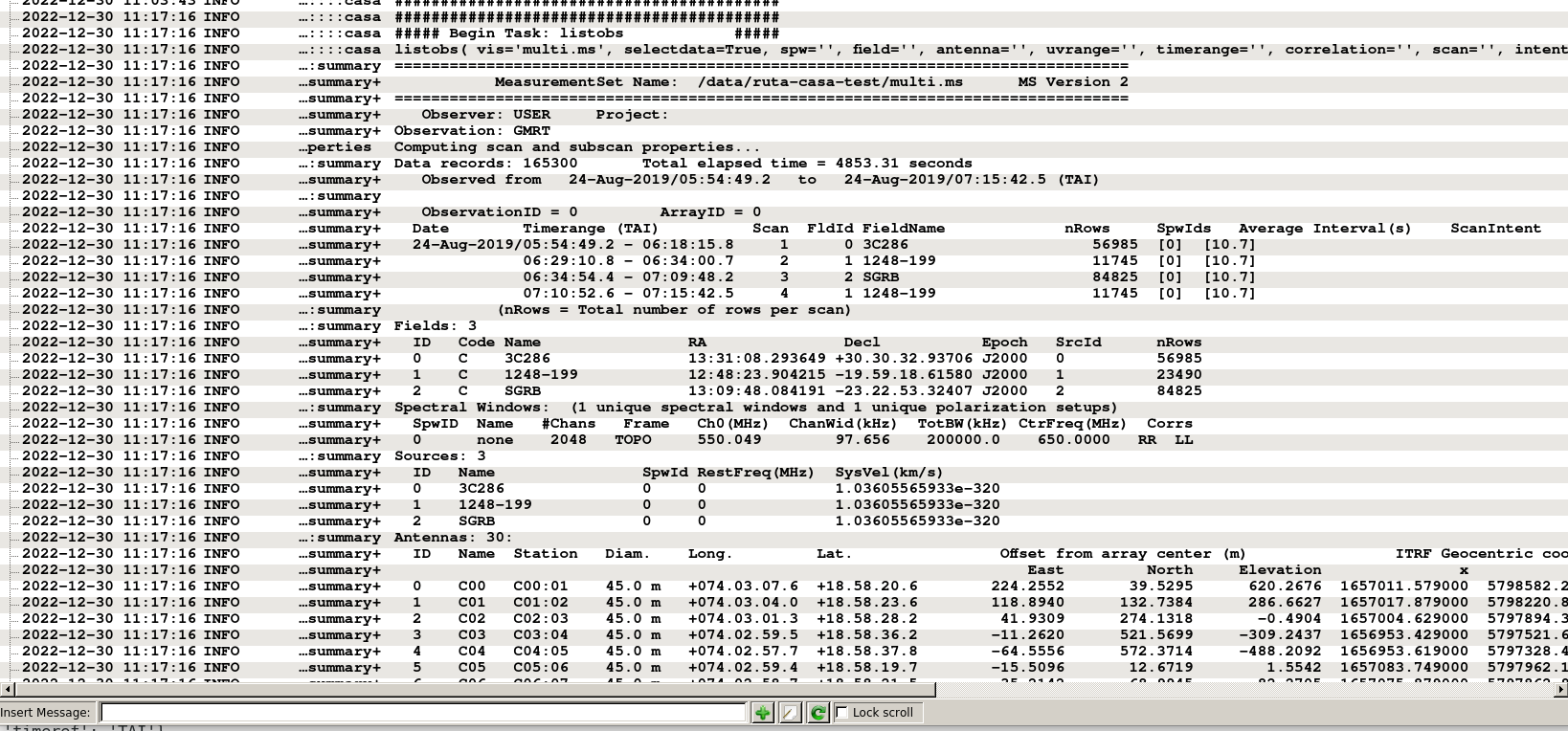
Output of the task listobs in the logger.

You can also choose to save the output to a text file so that you can refer to it when needed without having to run the task.

inp listobs
vis='multi.ms'
listfile='listobs-out.txt'
go listobs

Note the scans, field ids, source names, number of channels, total bandwidth, channel width and central frequency for your observations. Field ids (e. g. 0, 1, 2) can be used in subsequent task to choose sources instead of their names (e. g. 3C286, SGRB, etc.).

The task plotms is used to plot the data. It opens a GUI in which you can choose to display portions of your data. Go through the help for plotms GUI in CASA documentation.

It is important to make a good choice of parameters to plot, so that you do not end up asking to plot too much data at the same time - this can either lead to crashing of plotms or may take a long time to display the data.

Our aim is to inspect the data for non-working antennas. A good choice would be to limit the fields to calibrators and choosing a single channel and plot Amp Vs Time and iterating over antennas. Another good plot for inspection is to choose a single antenna, choose all the channels and plot Amp Vs Channel while iterating over baselines.

It is good to set the inputs for a task to default before running it.

default(plotms)
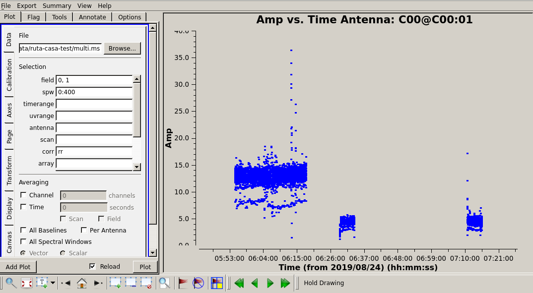
plotms

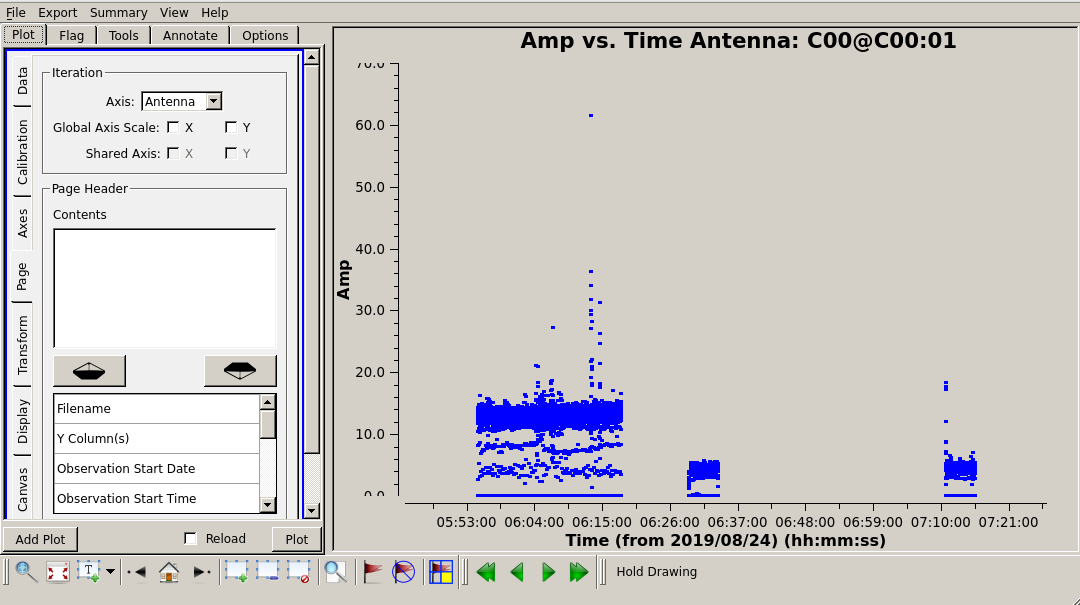
Screenshot of plotms. Fields 0 and 1 for the channel 400 and correlation rr are plotted for antenna C00. Iteration over anntennas in the Page tab seen on the left of the plotms window.

Flagging

Editing out bad data (e. g. non-working antennas, RFI affected channels, etc.) is termed as flagging. In our MS file, the bad data will be marked with flags and not actually removed as such - thus the term flagging. The task flagdata will be used to flag the data. See the detailed CASA documentation on flagging using the task flagdata.

Here some typical steps of flagging are outlined to get you started.

Usually the first spectral channel is saturated. Thus it is a good idea to flag the first spectral channel. The input ‘spw = 0:0’ sets the choice of spectral window 0, channel number 0.

default(flagdata)
inp flagdata
vis = 'multi.ms'
mode = 'manual'
spw = '0:0'
savepars = True
cmdreason = 'badchan'
go flagdata

Flagging the first and last records of all the scans is also similarly a good idea. Remember to set the task inputs to default before entering new inputs.

default(flagdata)
inp flagdata
vis = 'multi.ms'
mode = 'quack'
quackmode = 'beg'
quackinterval = 10
savepars = True
cmdreason ='quackbeg'
go flagdata

default(flagdata)
inp flagdata
vis = 'multi.ms'
mode = 'quack'
quackmode = 'endb'
quackinterval = 10
savepars = True
cmdreason ='quackend'
go flagdata

In the next step we would like to flag data on antennas that were not working. Using plotms, find out which antennas were not working. Non-working antennas generally show up as those having very small amplitude even on bright calibrators, show no relative change of amplitude for calibrators and target sources and the phases towards calibrator sources on any given baseline will be randomly distributed between -180 to 180 degreees. If such antennas are found in the data, those can be flagged using the task flagdata.

Note

Only an example is provided here - you need to locate the bad antennas in the tutorial data and flag those.

Remember also that the some antennas may not be bad at all times. However if an antennas stops working while on the target source, it can be difficult to find out. Thus make a decision based on the secondary calibrator scans. Depending on when such antennas stopped working, you can choose to flag them for that duration. Check the two polarizations separately.

Although plotms provides options for flagging data interactively, at this stage, we will choose to just locate the bad data and flag it using the task flagdata.

default(flagdata)
inp flagdata
vis = 'multi.ms'
mode = 'manual'
antenna = 'E02, S02, W06'
savepars = True
cmdreason = 'badant'
inp flagdata
go flagdata

It is a good idea to review the inputs to the task using (inp flagdata) before running it.

Radio Frequency Interferences (RFI) are the manmade radio band signals that enter the data and are unwanted. Signals such as those produced by satellites, aircraft communications are confined to narrow bands in the frequency and will appear as frequency channels that have very high amplitudes. It is not easy to remove the RFI from such channels and recover our astronomical signal. Thus we will flag the affected channels (may be individual or groups of channels). There are many ways to flag RFI - could be done manually after inspecting the spectra or using automated flaggers that look for outliers.

At this stage this will be done on the time-frequency plane for each baseline using the mode tfcrop in the task flagdata. In the first step we get an idea about the amount of flagging that will result from our choice of parameters action = 'calculate is the parameter that allows us to see this. Since we are still looking at uncalibrated data, we should be flagging only the worst RFI - the flagging percentage of a few percent is ok but if it shows high amount of flagging, one would like to increase the cutoffs used and check again. You may even decide to not use this automated flagger and examine the data further using plotms and locate the bad data and flag using manual mode in flagdata.

default(flagdata)
inp flagdata
vis = 'multi.ms'
mode = 'tfcrop'
spw  = ''
ntime = 'scan'
timecutoff =  6.0
freqcutoff = 6.0
extendflags = False
action = 'calculate'
display = 'both'
inp flagdata
go flagdata

If we are satisfied, we could run the same task with action = 'apply'.

default(flagdata)
inp flagdata
vis = 'multi.ms'
mode = 'tfcrop'
spw  = ''
ntime = 'scan'
timecutoff =  6.0
freqcutoff = 6.0
extendflags = False
action = 'apply'
display = ''
inp flagdata
go flagdata

Note

If you happen to wrongly flag and would like to restore the older flags, use the task flagmanager with mode = ‘list’ to see the flagbackup versions. Locate the version to which you want to restore and run flagmanager with mode =’restore’ providing the versionname. After that use the task flagmanager again with the to delete the unwanted flagbackup versions using it with mode =’delete’ and giving the unwanted versionnames.

Now we extend the flags (growtime 80 means if more than 80% is flagged then fully flag, change if required)

default(flagdata)
vis = 'multi.ms'
mode = 'extend'
growtime=80.0
growfreq=80.0
action='apply'
inp flagdata
go flagdata

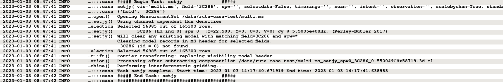
Absolute flux density calibration

In this step, flux densities are set for the standard flux calibrator in the data. The standard flux calibrators used at the GMRT are 3C286, 3C48 and 3C147. We can chose the flux density standard in this task. The default choice is Perlay-Butler 2017.

default(setjy)
vis = 'multi.ms'
field = '3C147'
go setjy

If more than one flux calibrators are present, run it for each of the sources.

Delay and bandpass calibration

First we will do delay calibration. In calibration, a reference antenna is required. Here “C00” is only taken as an example. You may use any antenna that is working for the whole duration of the observation. We will henceforth be using a central portion of the bandwidth. Depending on the shape of the band, you may change this selection.

default(gaincal)
vis = 'multi.ms'
caltable = 'multi.K1'
field ='3C286'
spw = '0:51~1950'
solint = '60s'
refant = 'C00'
solnorm = True
gaintype = 'K'
inp gaincal
go gaincal

An initial gain calibration will be done.

default(gaincal)
vis = 'multi.ms'
caltable = 'multi.G0'
field ='3C286'
spw = '0:51~1950'
solint = 'int'
refant = 'C00'
minsnr = 2.0
gaintype = 'G'
gaintable = ['multi.K1']
inp gaincal
go gaincal

Bandpass calibration using the flux calibrator.

default(bandpass)
vis = 'multi.ms'
caltable = 'multi.B1'
field ='3C286'
spw = '0:51~1950'
solint = 'inf'
refant = 'C00'
minsnr = 2.0
solnorm = True
gaintable = ['multi.K1','multi.G0']
inp bandpass
go bandpass

Examine the bandpass table using plotms. Choose the bandpass table multi.B1 in data and check the plots Amp Vs Channels and Phase Vs Channels iterated over antennas.

Note the shape of the band across the frequencies.

Gain calibration

A final gain calibration will be done in this step. The task gaincal will be run on the calibrators (flux calibrator/s, and gain calibrator/s).

default(gaincal)
vis = 'multi.ms'
caltable = 'multi.AP.G1'
field ='3C286'
spw = '0:51~1950'
solint = '120s'
refant = 'C00'
minsnr = 2.0
gaintype = 'G'
gaintable = ['multi.K1', 'multi.B1']
interp = ['nearest,nearestflag', 'nearest,nearestflag']\
inp gaincal
go gaincal

default(gaincal)
vis = 'multi.ms'
caltable = 'multi.AP.G1'
field ='1248-199'
spw = '0:51~1950'
solint = '120s'
refant = 'C00'
minsnr = 2.0
gaintype = 'G'
gaintable = ['multi.K1', 'multi.B1']
interp = ['nearest,nearestflag', 'nearest,nearestflag']
append = True
inp gaincal
go gaincal

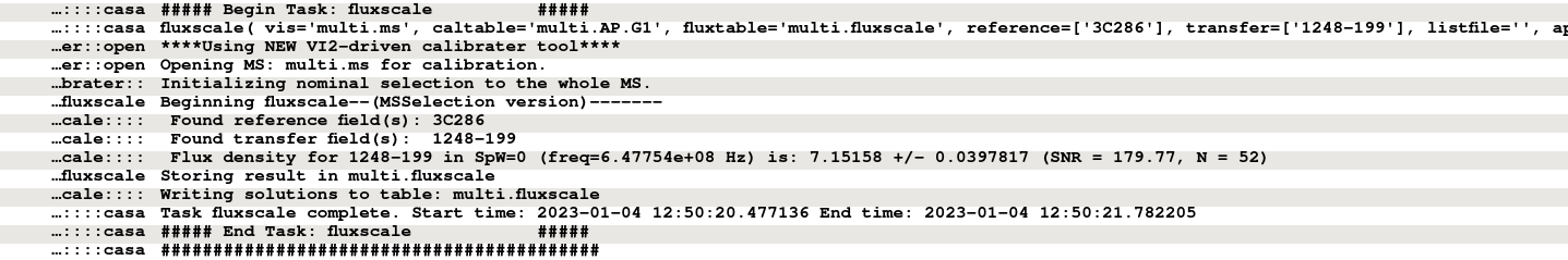
The flux density of the phase calibrator will be set in the following step.

default(fluxscale)
inp fluxscale
vis = 'multi.ms'
caltable = 'multi.AP.G1'
fluxtable = 'multi.fluxscale'
reference = '3C286'
transfer = '1248-199'
inp fluxscale
go fluxscale

Transfer of gain calibration to the target

First we apply the calibration to the amplitude and phase calibrators. This task creates the corrected data column in the MS file.

default(applycal)
inp applycal
vis='multi.ms'
field='3C286'
spw ='0:51~1950'
gaintable=['multi.fluxscale', 'multi.K1', 'multi.B1']
gainfield=['3C286','','']
interp=['nearest','','']
calwt=[False]
inp applycal
go applycal

default(applycal)
inp applycal
vis='multi.ms'
field='1248-199'
spw ='0:51~1950'
gaintable=['multi.fluxscale', 'multi.K1', 'multi.B1']
gainfield=['1248-199','','']
interp=['nearest','','']
calwt=[False]
inp applycal
go applycal

Apply calibration to the target.

default(applycal)
inp applycal
vis='multi.ms'
field='SGRB'
spw ='0:51~1950'
gaintable=['multi.fluxscale', 'multi.K1', 'multi.B1']
gainfield=['1248-199','','']
interp=['nearest','','']
calwt=[False]
inp applycal
go applycal

Use the task plotms to examine the calibrated data. You need to select corrected data column for plotting.

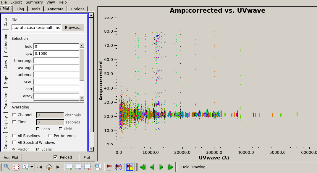
The calibrated Amp Vs UVwave for the flux calibrator.

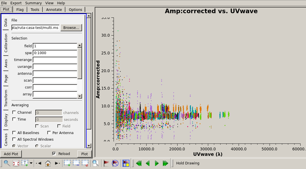
The calibrated Amp Vs UVwave for the calibrator 1248-199.

You will notice that there are some baselines showing higher amplitudes than the majority or some showing a large scatter.

Use plotms to locate which antennas and baselines have the outlier data. Use the task flagdata to flag those data.

Splitting the calibrated target source data

We will split the calibrated target source data to a new file and do the subsequent analysis on that file. Here we have chosen to drop some more of the edge channels.

default(mstransform)
inp mstransform
vis='multi.ms'
outputvis = 'SGRB-split.ms'
field='SGRB'
spw='0:201~1800'
datacolumn='corrected'
inp mstransform
go mstransform

Flagging on calibrated data

In this section flagging is done on calibrated target source data.

default(flagdata)
inp flagdata
vis = 'SGRB-split.ms'
mode = 'tfcrop'
timecutoff = 5.0
freqcutoff = 5.0
timefit = 'poly'
freqfit = 'line'
extendflags=False
inp flagdata
go flagdata

You may try out using window statistics and vary ntime to attain better flagging. Though always be careful about not overdoing the flags.

The mode rflag needs to be used with more caution. It is better to select uvranges where you expect the amplitudes to be comparable.

default(flagdata)
inp flagdata
vis='SGRB-split.ms'
mode="rflag"
uvrange = '>3klamda'
timedevscale=5.0
freqdevscale=5.0
spectralmax=500.0
extendflags=False
inp flagdata
go flagdata

Examine the data using plotms. Flag individual baselines as may be needed.

Averaging in frequency

The data are averaged in frequency to reduce the volume of the data. However the averaging is done only such that one is not affected by bandwidth smearing. For Band 4 it is recommended to average up to 10 channels (when BW is 200 MHz over 2048 channels). However in order to keep the computation time reasonable, for this tutorial we will average 20 channels. You can check the effect of this on the shapes of the sources at the edge of the field.

default(mstransform)
inp mstransform
vis='SGRB-split.ms'
outputvis='SGRB-avg-split.ms'
chanaverage=True
chanbin=20
inp mstransform
go mstransform

Some more flagging will be done on the data at this stage to get the final dataset for imaging. Use plotms to decide on where and what you would like to flag and proceed accordingly.

Imaging

We will use the task tclean for imaging. Go through the CASA documentation for tclean to understand the meaning of the various parameters. To save on computation, in this example we have set wprojplanes=128. In general to account for the w-term more accurately set wprojplanes= -1 so that it will be calculated internally in CASA. In this example we have used interactive = False in tclean.

default(tclean)
inp tclean
vis='SGRB-avg-split.ms'
imagename='SGRB-img'
imsize=7200
cell='1.0arcsec'
specmode='mfs'
gridder='wproject'
wprojplanes=128
pblimit=-0.0001
deconvolver='mtmfs'
nterms=2
weighting='briggs'
robust=0
niter=2000
threshold='0.01mJy'
cyclefactor = 0.5
interactive=False
usemask='auto-multithresh'
sidelobethreshold=2.0
pbmask=0.0
savemodel='modelcolumn'
inp tclean
go tclean

Keep an eye on the logger messages to get an idea about the processing and in particular see the total flux cleaned. Once the task ends successfully, you can view the image using imview. The main image you would like to see is the one with the extension image.tt0. Adjust the data range to display it in a reasonable colour scale to show the peaks as well as the noise in the image. Also inspect the rest of the images created by tclean - the .psf, .mask, .model, .residual.

imview

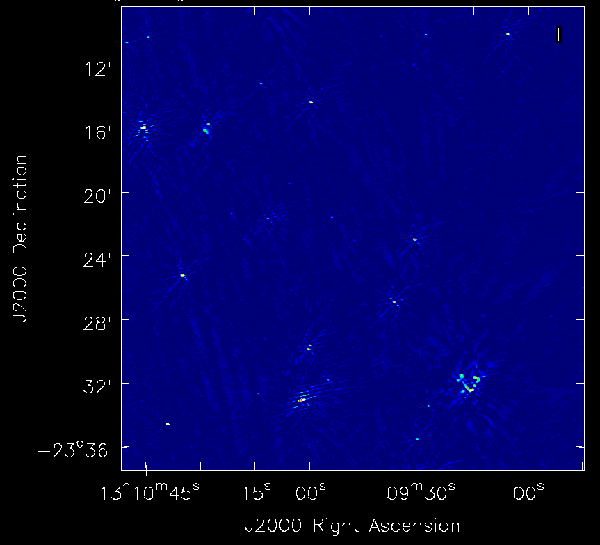
A zoom-in on the central region of the first image.

Self-calibration

This is an iterative process. The model from the first tclean is used to calibrate the data and the corrected data are then imaged to make a better model and the process is repeated. The order of the tasks is tclean, gaincal, applycal, tclean. A reasonable choice is to do 5 phase only and two amplitude and phase self-calibrations. We start from a longer “solint” (solution interval), for e. g. “8min” and gradually lower it to “1min” during the phase only iterations. For “a&p” self-calibration, again choose a longer solint such as “2min”. We keep solnorm=False in phase only iterations and solnorm=True in “a&p” self-calibration. As the iterations advance, the model sky is expected to get better so in the task tclean, lower the threshold and increase niter.

 default(gaincal)
 vis ='GRB-avg-split.ms'
 caltable='selcal-p1.GT'
 solint = '8min'
 refant ='C00'
 minsnr = 3.0
 gaintype = 'G'
 solnorm= False
 calmode ='p'
 go gaincal

Using the task "plotcal" you can examine the gain table. In successive iterations of self-calibration, you should find that the phases are more and more tightly scattered around zero. If this trend is not there, you can suspect that the self-calibration is not going well - check the previous tclean runs to see if the total cleaned flux was increasing.

default(applycal)
vis='SGRB-avg-split.ms'
gaintable='selcal-p1.GT'
applymode='calflag'
interp=['linear']
go applycal

We will split the corrected data to a new file and use it for imaging. This is just for better book-keeping. You may choose to do the successive self-calibration iterations on the same MS file but remember that the corrected data and model data columns will be overwritten by applycal and tclean.

default(mstransform)
vis='SGRB-avg-split.ms'
datacolumn='corrected'
outputvis='vis-selfcal-p1.ms'
go mstransform

In the next iteration we will use a larger niter and lower the threshold. In the tclean messages do check the total cleaned flux and the number of iterations needed to reach that.

default(tclean)
imagename='SGRB-img1'
imsize=7200
cell='1.0arcsec'
specmode='mfs'
gridder='wproject'
wprojplanes=128
pblimit=-0.0001
deconvolver='mtmfs'
nterms=2
weighting='briggs'
robust=0
niter=4000
threshold='0.01mJy'
cyclefactor = 0.5
interactive=False
usemask='auto-multithresh'
sidelobethreshold=2.0
pbmask=0.0
savemodel='modelcolumn'
inp tclean
go tclean

Repeat until you stop seeing improvement in the image sensitivity.

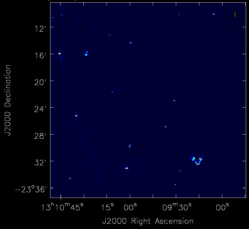
A zoom-in on the central region of the image after self-calibration.

After you get your final image you need to do a primary beam correction. The task “widebandpbcor” in CASA does not have the information of the GMRT primary beam shape. A modified version of this task called ugmrtpb has been written for the uGMRT primary beam correction. You can follow the instructions there to do a primary beam correction for your image.

For this tutorial on the RAS machines please see the steps here.

Acknowledgements: We thank Ishwara Chandra who provided the data used in the Radio Astronomy School for the CASA tutorial. We also thank Nissim Kanekar and Ruta Kale who helped make the first version of this tutorial. The original tutorial has been converted to html by Ruta Kale with help from Shilkumar Meshram.