Pulsar data analysis

The tutorial is intended to provide you a basic introduction to the steps involved in the analysis of pulsar data, including searching for new giant-pulses/transient events from pulsars and timing a newly discovered pulsar. The filterbank data obtained from GMRT are converted to SIGPROC filterbank format using either the filterbank command from SIGPROC or the rficlean command from RFIClean. The tutorial will use data already converted to the SIGPROC filterbank format.

Prerequisite

You need to have PRESTO, SIGPROC, TEMPO2, TEMPO, and their dependencies installed on your machine. You also need the SIGPROC filterbank data to be available on your disk.

Pulsar General Data Analysis

This part of the tutorial aims to demonstrate the process of pulsar detection and determining its properties using observations from GMRT. We will use band-4 (550-750 MHz) data of a test pulsar.

Introduction

You need to have PRESTO, SIGPROC, TEMPO2, TEMPO, and their dependencies installed on your machine. You also need the SIGPROC filterbank data to be available on your disk.

The header information of the data from a SIGPROC filterbank file can be inspected using the readfile command (shown below) from PRESTO or the header command from SIGPROC.

readfile B1133+16_b4_rficlean_digifil.fil

Example of a filterbank header

Data inspection

A section of the raw data can be inspected by plotting the data as a function of time and frequency, e.g., using the waterfaller.py command from PRESTO. The command waterfaller.py has several provisions that enable inspecting the data in several ways (e.g., before and after dedispersion, partial and full averaging over the bandwidth, etc.)

waterfaller.py B1133+16_b4_rficlean_digifil.fil -T 126.4 -t 0.3 --show-ts

The sweep across the frequencies is caused by the propagation effects of the medium. Due to the frequency-dependent refractive index, signal at higher frequencies reach earlier compared to its counterpart at the lower frequencies. The time delay depends on the electron column density along the line of sight (dispersion measure or DM), and can be corrected if the DM is known.

waterfaller.py B1133+16_b4_rficlean_digifil.fil -T 126.4 -t 0.3 -d 4.84 --show-ts

Dedispered Time Series

A small section of data can be dedispersed and viewed using waterfaller.py as seen above. To get the dedispersed timeseries for the whole data we will use prepdata from PRESTO. For an unknown pulsar, prepsubband can be used to dedisperse the filterbank file at multiple trial DM values.

prepdata -nobary -o B1133+16_b4_rficlean_digifil -dm 4.840 B1133+16_b4_rficlean_digifil.fil

Exploring the time series

Now, since we have the dedispersed time series, we can try to visualize the pulses in the time series. Use exploredat to visualize the time series,

exploredat B1133+16_b4_rficlean_digifil.dat

This will generate an interactive plot,

Output plot of exploredat. One can zoom in, zoom out, and move around in this plot.

Single pulse search

Though we have seen the single pulses from the pulsar directly in the time series, there is a formal way to search for single pulses in the time series.

single_pulse_search.py -t <significance_threshold> -m <maximum_width> <dedispersed_time_Series.dat>

Output of single pulse search. We get the location of pulses, number of pulses, and single pulse S/Ns as a function of DM.

You can note down the timestamp of some strong pulses from the text file and try to verify its presence in the time series using exploredat.

Folding Process

There are pulsars that are weak and can not be seen in single pulses. To recover such pulsars, we use their periodic property to get a good indication of their presence in the time series. Once the period, period derivative, and higher order period derivatives (if any) for the pulsar are known, the time stamp array (in mjd) is wrapped around that period (also accounting for any changes in the period with time due to its higher derivatives). This process of wrapping the time sample and adding the intensities at the corresponding spin-phases of the pulsar is known as folding the data.

Folding filterbank file

Once we know the correct period and DM of the pulsar, we can fold the filterbank file to generate characteristic plots of the pulsar. We use prepfold to fold a filterbank,

prepfold -p <period> -dm <DM> -nosearch -zerodm <filterbank_file.fil>

Result of prepfold. Profile of the pulsar along with subintegration vs phase, frequency vs phase, S/N vs DM, S/N vs period plots.

Once the pulsar is detected, one can find out other properties of the pulsar (duty cycle, flux density, scintillation, etc). as explained below.

Flux determination

From the telescope, we obtain a intensity time series (corresponding to the Electric field of radio emission from the source of interest from the sky) in arbitrary units. These arbitrary unit values are then converted to Jansky (Jy) units. For this, we need to know the conversion factor of noise fluctuation (of the blank sky) of the radio telescope. This is already done by the observatory and is given in the form of T_sys/G as a function of radio frequency.

The equation to be used is known as the radiometer equation.

Flux (in Jansky) = SNR x RMS,

where

RMS (Jansky) = [T_sys/(G x Antenna factor)] x [1/sqrt(nPol x bandwidth x duration)] x sqrt[W/(P-W)],

and SNR is the ratio of signal to noise (i.e., a unitless quantity). T_sys is the antenna temperature (Kelvin; K) and G is the gain of each antenna which has units of K/Jy, nPol is the number of polarizations, and W and P are the pulse width and the period of pulsar, respectively.

Antenna factor in the above formula depends on the type of beam used (IA: incoherent array or PA: phased array). For PA the value of antenna factor would be the total number of antennas (N), in the case of IA the value is sqrt(N).

Scintillation

The radio waves (EM waves) emitted from the source, pass through the interstellar medium (ISM) and earth’s ionosphere. The difference between the refractive indices of the medium between the source and observer causes the phases of the EM wave to modulate. This causes a scope of interference between the EM waves with slightly different relative phases (traveling through LOS very close to the source’s direction) and causes constructive and destructive interference patterns. Observationally, this interference pattern injects modulation of the observed flux density (in the form of dynamic spectra). This constructive and destructive interference is seen in timescales of a few seconds to a few hours, and this type of scintillation is called diffractive scintillation.

The other type of scintillation which has timescales of few months to years, is called refractive scintillation. These are caused by changes in the large refractive index of the intervening medium, which in turn causes to focus/defocus the rays of light emitted from the source.

Radius to Frequency Mapping (RFM)

Pulsars have a magnetosphere extended up to the light cylinder, which comprises highly magnetized plasma flowing outwards. Considering the dipolar magnetic field, the plasma generated in an electric gap near the surface, pair-cascades and flows along the open field lines. The profile of the pulsar at a given observing frequency represents emission from a corresponding range of emission heights. The plasma in the magnetosphere emits in the radio regime, by the process of coherent curvature radiation (CCR). As per the theory of CCR, different frequencies are emitted at different heights (distance from the surface of the neutron star). This coupled with the multi-component profile ultimately creates a shift in the relative position of different components of the profile. This phenomenon is called the Radius-to-Frequency Mapping.

Timing of Pulsars

The tutorial is intended to provide you an introduction to the basic steps related to the timing analysis of pulsar using GMRT and Parkes beam data. We will be using uGMRT Band-3 data centered at 400 MHz with a 200 MHz bandwidth, as well as Parkes data centered at 1440 MHz with a 128 MHz bandwidth. We will consider the case of an binary pulsar for the exercise.

We will use PRESTO and TEMPO2 Softwares.

Introduction

The beam data is in binary format and is converted to “filterbank” format (same binary file with a header). The “filterbank” is folded based on pulsar ephemeris, yielding three-dimensional (time, frequency, phase) folded pulsar data (“pfd”). For this tutorial, we will begin with “pfd” files.

You need to have PRESTO and TEMPO2 installed on your machine. You also need the “pfd” files to be available on your disk.

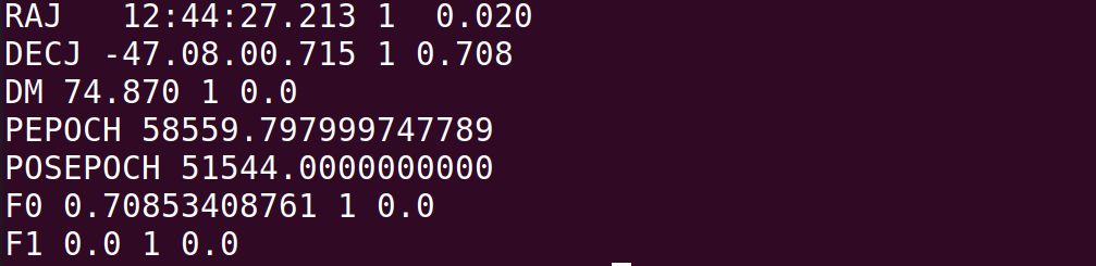
Prediction of phases of pulsar using TEMPO2

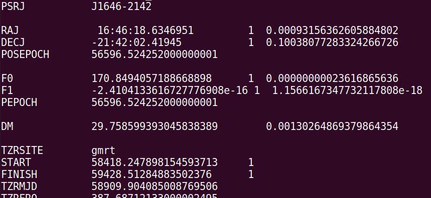
Right Ascension (RA) and Declination (DEC) provide the source’s two-dimensional position in the sky, typically defined using the J2000 system. The pulsar’s spin frequency (F0) is the reciprocal of its spin period, and F1 is the first derivative of the spin frequency with respect to time. Since pulsars gradually slow down, F1 is negative. The dispersion measure (DM) quantifies the line-of-sight electron column density. To account for the pulsar’s motion relative to Earth, we use proper motion parameters: PMRA (proper motion in right ascension) and PMDEC (proper motion in declination). Parallax (PX) represents the apparent shift in the pulsar’s position due to Earth’s orbit around the Sun. For pulsars in binary systems, we also have additional binary orbital parameters: orbital period (PB), sine of the binary inclination angle (SINI), projected semimajor axis (A1), epoch of periastron passage (T0), longitude of periastron (OM), eccentricity (ECC), and companion mass (M2). Due to long-term changes in the pulsar’s orbit, variations in orbital period (PBDOT) and longitude of periastron (OMDOT) can also be observed. All these parameters are stored in the pulsar’s parameter file. Let’s start with the parameter file of pulsar J0437-4715, which includes the pulsar’s name, RA, DEC, F0, F1, DM, PMRA, PMDEC, PX and the above mentioned binary parameters. Using this parameters file we can predict the ToAs of the future pulses.

cat J0437-4715.par

cat J0437-4715.tim

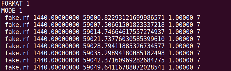
This file “J0437-4715.tim” contains the observed times of arrival (ToAs) of the pulses for this pulsar ranging from MJD 49350 to 53000 and is generated using the “get_TOAs.py” script of PRESTO.

tempo2 -gr plk J0437-4715.par J0437-4715.tim

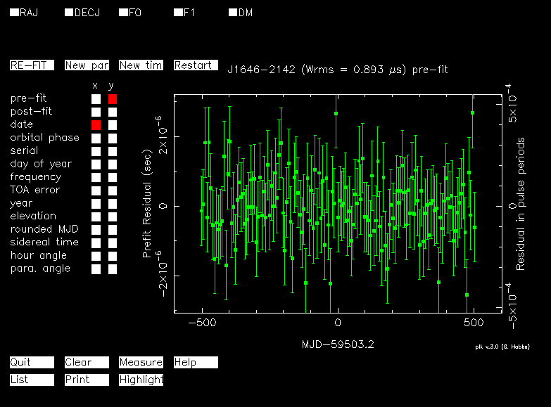
This is the graphical user interface of tempo2. The plot shows timing residuals on the y-axis and time as Modified Julian Date (MJD) on the x-axis. Timing residuals represent the difference between observed and predicted times of arrival (ToAs). Ideally, the residuals should cluster around zero, leaving only Gaussian noise. However, small errors in parameter values can introduce patterns in the timing residuals, which we will explore in the next section.

The impact of parameter errors on timing data

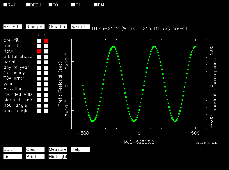
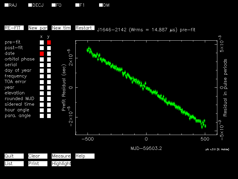
Now let’s introduce a small error (say around an arc-sec) in postion (RA and DEC) in the parameter file to see the effect of wrong position on the timing data. After putting the offset in the parameter file, run the above command again which will show that an error in position has yearly periodic variation in the residuals. This is demonstrated in figure below.

If you fit for the RA/DEC for which the error is introduced, you will again get the randomly sampled residuals around the zero line in the post-fit residuals.

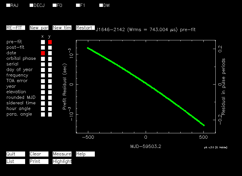
Now, reset the parameter file to its default values and try introducing a small error in F0. The residuals for the F0 error show a straight line pattern with no periodicity, as shown below.

Again, if you fit for F0, you will get the randomly sampled residuals around the zero line in the post-fit residuals.

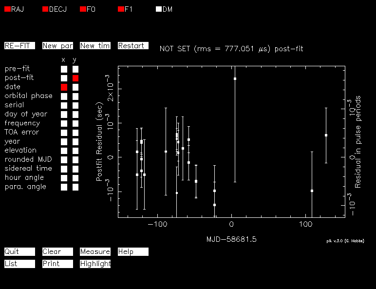
Try the same thing again with error in F1, and this time you’ll notice a parabolic long-term variation like the one in the image below.

Understanding the pattern in the residuals caused by parameter error will assist us in solving a newly discovered pulsar. Once accurate (phase-coherent) solutions for a pulsar are obtained, one can establish its clock-like behaviour and predict its phases at any point in time.

Time to solve a Newly Discovered Pulsar

This time we will start with the GMRT data set for a newly discovered binary millisecond pulsar J1242-4712 which is discovered in the GMRT High Resolution Southern Sky Survey.

This pulsar was localised through imaging of a single observational epoch which provides us with its RA and DEC which are accurate to a few arc-seconds. The F0 and DM values of the pulsar were estimated using data from an epoch observation in which the pulsar was strongly detected. We used the reciprocal of the period value (in seconds) given in the waterfall plot of that observation to calculate F0. Similarly, from the same plot, we noted the DM and epoch of the observation. To get an initial guess for the binary parameters we use the following routine of presto, which uses non-linear least-squares optimizer for solving pulsar orbits

fitorb.py [-p p] [-pb pb] [-x x] [-T0 T0] [-e e]  bestprof_files

Using these values, we created a parameter file for this pulsar (in this case, J1242-4712_initial.par) that contains an initial guess of its parameters.

cat J1242-4712_initial.par

In this exercise, we will use GMRT’s incoherent array (IA) beam data. The GMRT IA beam data is first converted to “filterbank” format, then dedispersed and folded to “pfd” format. We’ll start with the “pfd” files right away.

Time of arrival estimation

The “pfd.ps” files contain waterfall plots for all “pfd” files. The first step is to go through all of the profiles and find the cleanest one with the sufficiently bright integrated pulse. We will use that profile as our reference or template profile, assuming it is the true profile of the pulsar. Use the following command to view all the profiles.

evince *ps

After selecting the template profile, the next step is to estimate how many ToAs should be extracted from each observation. We will derive a single ToA for full observation for weak detections, two ToAs for mildly detectect profiles, and four ToAs for bright detections. This approach will be adequate to find the solution in this specific case. To determine the number of ToAs for individual observations, check all the profiles again using the command above.

Let’s say you’ve selected k ToAs for a particular observation A.pfd and B.pfd is your chosen epoch for the template. Then run the following command to get the ToAs for observation A.pfd.

get_TOAs.py -n k -t B.bestprof A.pfd >> J1242-4712.tim

This command will find the ToAs for observation A.pfd by cross-correlating it with template B.bestprof. The ToAs will be saved in the J1242-4712.tim timing file.

The value of k varies depending on the detection strength of the pulsar for each observation. So, for each observation, use the same command, but change the file names A.pfd and the corresponding k value while keeping the template same (i.e., B.bestprof). Once all observations’ ToAs have been generated, run the command below.

tempo2 -nofit -f J1242-4712_initial.par J1242-4712.tim -gr plk

This command displays the difference (or residuals) between the observed ToAs (in the J1242-4712.tim file) and the predicted ToAs (predicted using J1242-4712_initial.par file). Because the ToAs for a newly discovered pulsar are not phase-connected, we will not see any general systematic pattern in the residuals. This is illustrated in the figure below.

Now, take a sample of densely sampled points and start fitting from F0. Once you’ve identified a pattern in the ToAs, try fitting RA and DEC. Finally, you can try fitting F1, but keep in mind that the value of F1 for 9 months of data will be highly unreliable. Once phase coherent solutions are obtained, ToAs will exhibit near-random behaviour around the zero line, as shown in the figure below.

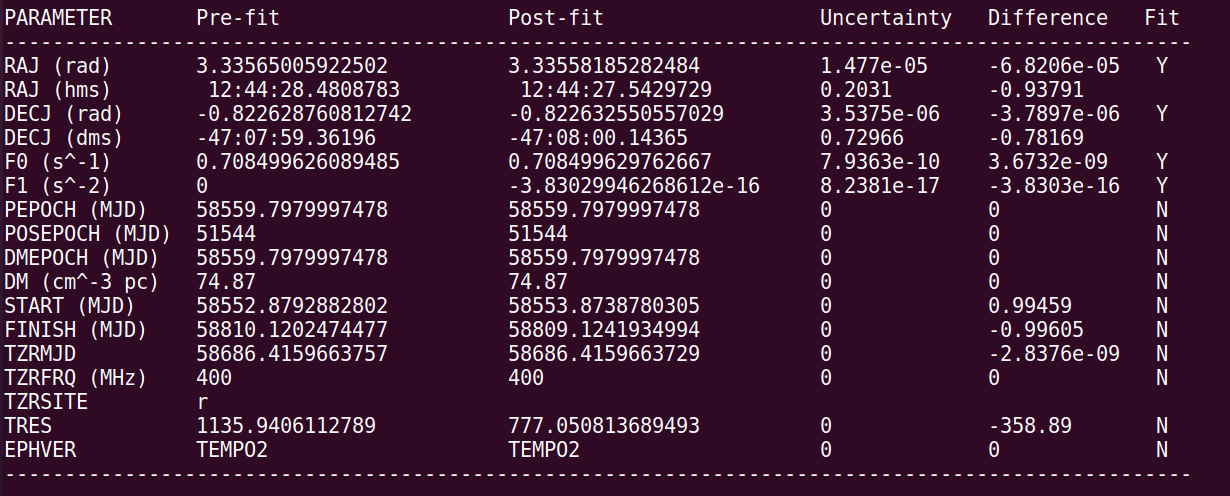
Examine the F0, F1, RA, and DEC values. Since RA and DEC are obtained through imaging, the post-fit RA and DEC should be within a few arc-seconds of the initial guess (i.e., pre-fit values). The F1 value after fitting should be negative and small (compared to error in F0). Below are the fitted values for this exercise.

Finally, on the graphical interface, select “new par” to create the new parameter file. Now that the pulsar’s phase-coherent solution has been found, you will be able to predict the ToAs in future observations. The prediction accuracy improves as the number of observations and the timing baseline increase.

Acknowledgements and Credits

The Pulsar General Data Analysis section is contributed by Banshi Lal and Rahul Sharan, and the Timing of pulsars section is contributed by Ankita Ghosh and Sangita Kumari. The data sets used in the latter are kindly provided by Ankita Ghosh. Yogesh Maan is responsible for the overall pulsar tutorial coordination.